
If you have ever spent an afternoon copying data from one spreadsheet to another, deleting blank rows, fixing date formats, and silently bargaining with the universe, Power Query is the Excel feature you wish you had met earlier. In Excel 2016, Power Query is not a mysterious secret add-in hiding in a digital cave. It is built into Excel under a friendlier name: Get & Transform.
This guide explains exactly how to activate Power Query in Excel 2016, where to find it, what to do if it is missing, and how to test that it works. Whether you are cleaning sales reports, combining monthly files, importing CSV data, or preparing a dashboard, Power Query can turn repetitive spreadsheet chores into refreshable workflows. In other words, it is the difference between “I’ll fix this again next Monday” and “Excel, please do the thing.”
Below are nine practical steps to help you enable, locate, and start using Power Query in Excel 2016 on Windows.
What Is Power Query in Excel 2016?
Power Query is Excel’s data import, cleanup, and transformation tool. It lets you connect to data from workbooks, text files, CSV files, databases, web pages, folders, and other sources. Once connected, you can remove columns, filter rows, split text, merge tables, change data types, and reshape messy information without manually editing the original file.
In Excel 2016, Microsoft integrated Power Query directly into the ribbon as Get & Transform. That means most Excel 2016 users do not need to download a separate Power Query add-in. If you are looking for a tab named “Power Query,” you may not find one. Look for the Data tab instead, then find the Get & Transform group.
This small naming detail causes a lot of confusion. Users often think Power Query is missing when it is actually sitting right there on the Data tab, wearing a different name like it is trying to avoid awkward small talk at a party.
Before You Start: What You Need
To follow this tutorial, you should have:
- Microsoft Excel 2016 for Windows
- A working Excel installation with access to the ribbon menu
- Permission to update or modify Office settings if commands are missing
- A sample file, such as a CSV or another Excel workbook, for testing
Power Query is most complete in the Windows version of Excel 2016. Some features may vary depending on your Office edition, update status, and installation type. If you are using Excel 2016 for Mac, your available Power Query features may be more limited than the Windows version.
How to Activate Power Query in Excel 2016: 9 Steps
Step 1: Open Excel 2016
Start by opening Microsoft Excel 2016. You can launch it from the Start menu, desktop shortcut, taskbar, or by opening any Excel workbook. Once Excel is open, create a blank workbook so you can safely explore the ribbon without changing an existing file.
This step sounds obvious, but it matters because Power Query is accessed from inside Excel, not from a separate desktop program. In Excel 2016, Power Query works as part of the workbook environment. You import data, transform it in the Power Query Editor, and then load the results back into Excel.
Step 2: Go to the Data Tab
Look at the ribbon across the top of the Excel window and click the Data tab. This is where Excel 2016 keeps its data import and connection tools.
On the Data tab, look for a section called Get & Transform or Get & Transform Data. This is Power Query. You may see commands such as:
- Get Data
- New Query
- From Table/Range
- From Text/CSV
- Recent Sources
- Existing Connections
If you see these options, congratulations. Power Query is already activated in Excel 2016. No dramatic installation ceremony required.
Step 3: Make Sure the Data Tab Is Visible
If you do not see the Data tab, it may be hidden from your ribbon. To bring it back, click File, then choose Options. In the Excel Options window, select Customize Ribbon.
On the right side, under Main Tabs, look for Data. Make sure the checkbox beside Data is selected. Then click OK.
Return to the ribbon and check again. The Data tab should now appear. This does not install Power Query, but it restores the ribbon area where Power Query tools live.
Step 4: Locate the Get & Transform Group
Once the Data tab is visible, look carefully for the Get & Transform group. Depending on your screen size, Excel window width, and Office update version, the commands may appear slightly differently. On a smaller screen, some buttons may collapse into drop-down menus.
Try widening the Excel window if you cannot see the full ribbon. You can also click small arrows or grouped command buttons to expand hidden options. In many Excel 2016 installations, Power Query commands appear under Get Data or New Query.
The key point is simple: in Excel 2016, “Power Query” and “Get & Transform” refer to the same general feature set for importing and shaping data.
Step 5: Update Excel 2016 If Power Query Commands Are Missing
If the Data tab is visible but the Get & Transform tools are missing or very limited, your Office installation may need updates. Excel 2016 received updates that improved and expanded Get & Transform features, so an outdated build can look different from tutorials you find online.
To check for updates, click File, then select Account. Look for Office Updates and choose Update Options. Click Update Now if the option is available.
If your workplace manages Office updates, you may not see this option. In that case, contact your IT administrator and ask whether Excel 2016 can be updated to include the full Get & Transform experience. That sentence may not sound exciting, but it can save you from clicking around Excel like you are searching for buried treasure.
Step 6: Check Disabled Items
If Power Query or related data tools still do not appear, check whether Excel has disabled an item after a crash or startup problem. Go to File, then Options, and choose Add-ins.
At the bottom of the window, find the Manage drop-down menu. Select Disabled Items, then click Go. If you see any Microsoft data add-ins or related Excel components listed there, select them and click Enable.
In many cases, Power Query will not appear as a separate add-in in Excel 2016 because it is integrated into Excel. Still, checking Disabled Items is a smart troubleshooting step when ribbon tools disappear unexpectedly.
Step 7: Review COM Add-ins If Needed
Next, return to File > Options > Add-ins. This time, use the Manage drop-down menu to select COM Add-ins, then click Go.
In Excel 2016, you may not see a separate “Microsoft Power Query for Excel” checkbox. That is normal. Power Query was a downloadable add-in for older versions such as Excel 2010 and Excel 2013, but Excel 2016 generally includes it as part of the Data tab experience.
If you do see a relevant Microsoft Power Query option, make sure it is checked, then click OK. If you do not see one, do not panic. Return to the Data tab and continue checking for Get & Transform commands.
Step 8: Test Power Query with From Table/Range
The easiest way to confirm that Power Query is working is to test it with a simple table. In a blank worksheet, type a small data set such as this:
| Product | Region | Sales |
|---|---|---|
| Desk Lamp | East | 120 |
| Office Chair | West | 340 |
| Notebook | South | 80 |
Select any cell in the data range. Then go to Data > From Table/Range. Excel may ask whether your table has headers. Confirm the option if your first row contains column names, then click OK.
If the Power Query Editor opens, Power Query is active. You can now transform the data. For example, you can filter the Region column, change the Sales column to a number format, remove unnecessary columns, or rename headers.
Step 9: Load the Query Back into Excel
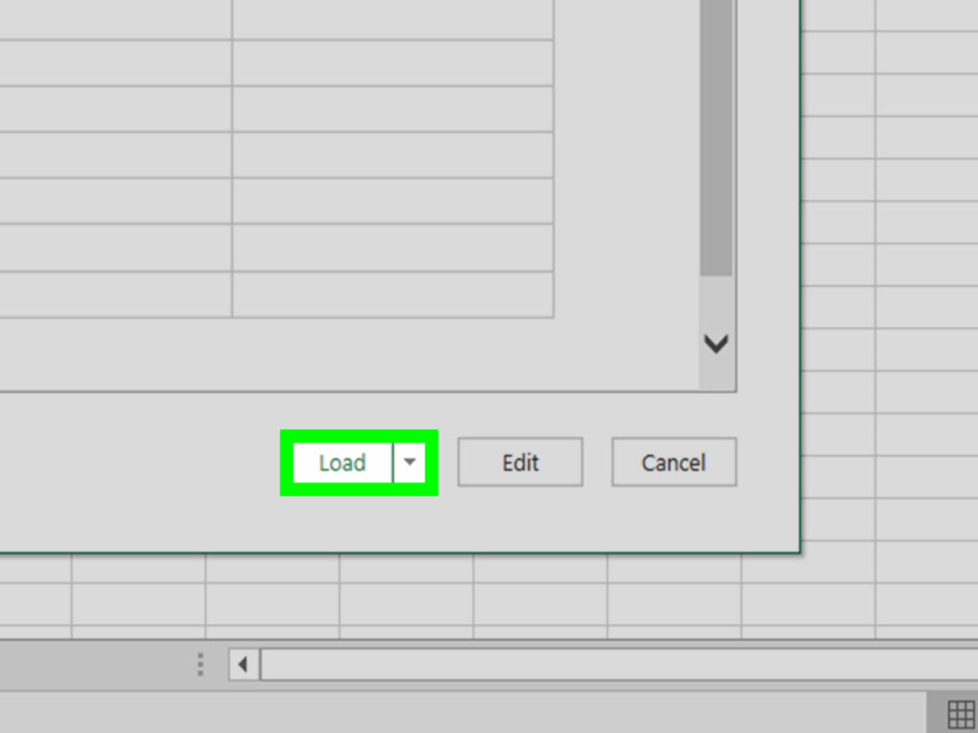
After testing a few transformations, click Close & Load in the Power Query Editor. Excel will load the cleaned data into a worksheet as a table. This confirms that Power Query is not only visible but functioning properly.
From now on, you can refresh the query instead of repeating the same cleanup steps manually. If the source data changes, right-click the output table and choose Refresh. Excel will rerun the saved Power Query steps. It is like teaching Excel a recipe once and then letting it cook the same meal every time, minus the dishes.
Common Problems When Activating Power Query in Excel 2016
Power Query Is Missing from the Ribbon
If Power Query appears to be missing, remember to look for Get & Transform on the Data tab. Excel 2016 does not always display a separate Power Query tab. If the Data tab itself is missing, restore it through File > Options > Customize Ribbon.
The Get Data Button Looks Different
Excel 2016 has changed over time through updates. Some versions show New Query, while others show Get Data. The available connectors may also vary. For example, newer versions of Excel may include connectors that older Excel 2016 builds do not have.
Power Query Is Not Available on Mac the Same Way
If you are using Excel 2016 for Mac, the Power Query experience may not match Excel 2016 for Windows. Many tutorials are written for Windows, so Mac users may see fewer options or different menus. For the most complete Power Query workflow in Excel, Windows versions traditionally provide the broader feature set.
Your Organization Controls Office Updates
In a business or school environment, Office updates may be managed by an administrator. If you cannot update Excel yourself, ask IT whether your Office 2016 build supports the Get & Transform features you need. Mentioning “Power Query” and “Get & Transform” together helps avoid confusion.
Why Activate Power Query in Excel 2016?
Power Query is useful because it turns manual cleanup into a repeatable process. Instead of fixing the same messy file every week, you build a query once and refresh it whenever new data arrives.
Here are a few practical examples:
- Combine monthly reports: Import files from a folder and append them into one table.
- Clean CSV exports: Remove blank rows, fix headers, and change data types before analysis.
- Prepare dashboard data: Shape raw data before loading it into PivotTables or charts.
- Split messy columns: Separate full names, product codes, or location fields into cleaner columns.
- Merge lookup tables: Join sales data with product, customer, or region information.
For anyone who works with recurring reports, Power Query can save hours. It also reduces errors because the same transformation steps are applied consistently each time.
Best Practices After Activating Power Query
Use Clear Query Names
Rename your queries so they describe what they do. Names like Cleaned_Sales_Data or Monthly_Report_Combined are much easier to understand than Query1, Query2, and the mysterious Query2_Final_REAL_Final.
Check Data Types Early
Power Query assigns data types such as text, number, date, and currency. Always check these early in your workflow. A date stored as text can cause sorting, filtering, and calculations to behave strangely.
Keep Source Files Organized
If your query imports from a folder, keep file names and column structures consistent. Power Query is powerful, but it is not a mind reader. If one file has “Sales Amount” and another has “Revenue Total,” you may need extra cleanup steps.
Refresh Before Reporting
Before sharing a report, refresh your queries. Go to the Data tab and use Refresh All. This ensures your workbook reflects the latest available source data.
Experience Notes: What It Is Really Like to Use Power Query in Excel 2016
After working with Power Query in Excel 2016, one of the biggest lessons is that the hardest part is often not the tool itself. The hard part is understanding what your data is doing before it reaches Excel. Power Query can clean up a lot, but it rewards users who take a few minutes to inspect their source files first.
For example, imagine you receive a weekly sales report from five regional managers. Each manager sends an Excel file. The columns are supposed to be the same, but one person writes “Sales Rep,” another writes “Representative,” and someone else adds a cheerful extra column called “Notes from Jim.” Without Power Query, you may spend time copying, pasting, deleting, and reformatting. With Power Query, you can build a process to import the files, standardize the columns, remove unnecessary fields, and combine everything into one clean table.
The first time you build a query, it may feel slower than doing the work manually. That is normal. You are not just cleaning one report; you are creating a reusable cleanup machine. The payoff arrives the second, third, and tenth time you need the same report. Instead of repeating the entire process, you refresh the query and let Excel apply your saved steps.
A good habit is to make one change at a time in the Power Query Editor and watch the Applied Steps pane on the right. Every action becomes a recorded step. If something breaks, you can click earlier steps to find where the problem started. This is much better than traditional spreadsheet editing, where one accidental paste can turn a neat workbook into modern art.
Another useful experience tip is to avoid overloading your workbook. Power Query can handle a lot, but Excel workbooks can still become slow if you load huge tables directly to worksheets. When possible, load only the final cleaned result you need. If you are preparing data for PivotTables or models, consider connection-only queries where appropriate.
It is also smart to document your process. Add short, clear query names and keep a small notes sheet in the workbook explaining where the source data comes from, how to refresh it, and what each query does. Future you will appreciate this. Future you may even send present you a thank-you card, although Excel has not yet added that feature.
Power Query in Excel 2016 is especially helpful for users who are not programmers but still need reliable automation. You do not need to write complex code to remove rows, merge tables, split columns, or replace values. The interface lets you perform many transformations by clicking buttons. Behind the scenes, Power Query records those actions in its own formula language, but beginners can get real value without touching the code.
The most important mindset is this: do not use Power Query only when your data is already beautiful. Use it when your data is repetitive, annoying, inconsistent, or delivered in a format that makes you sigh. That is exactly where Power Query shines. Excel 2016 may not have every modern connector found in newer versions, but its Get & Transform tools are still strong enough for many everyday business tasks.
Conclusion
Activating Power Query in Excel 2016 is usually less about installing something new and more about knowing where Microsoft placed it. In Excel 2016 for Windows, Power Query is built into the Data tab as Get & Transform. If you can see that group, you are ready to import, clean, transform, and refresh data like a spreadsheet wizard with a very practical hat.
If the tools are missing, check whether the Data tab is hidden, update Office, review disabled items, and inspect add-in settings. Once Power Query is available, test it with From Table/Range, open the Power Query Editor, make a simple change, and load the result back into Excel.
Power Query is one of the most useful features in Excel 2016 because it helps replace repetitive manual cleanup with repeatable steps. For reports, dashboards, CSV files, folder imports, and messy business data, it can save time, reduce errors, and make Excel feel much less like a punishment from the spreadsheet gods.
SEO Tags
Note: This article is written for Excel 2016 users, especially on Windows, where Power Query appears as Get & Transform on the Data tab. Menu names and available connectors may vary depending on your Office build, update channel, and organization settings.