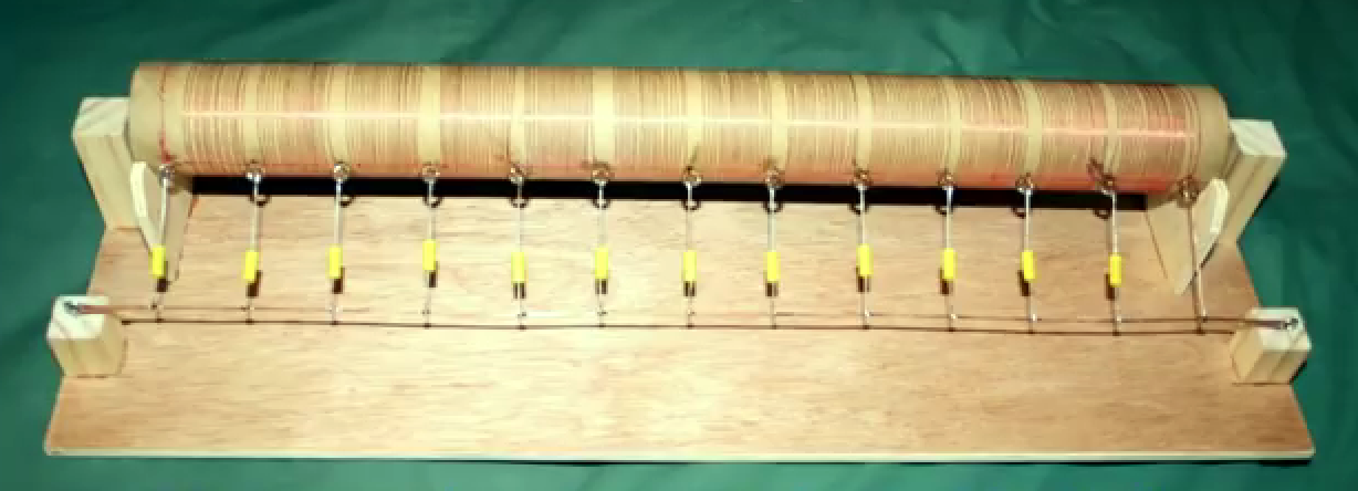

A model of a transmission line is one of those engineering ideas that looks innocent at firstjust a wire, right? Then physics walks in wearing safety boots and says, “Actually, we need resistance, inductance, capacitance, conductance, wave propagation, reflections, delay, losses, voltage regulation, and maybe a cup of coffee.” In electrical engineering, a transmission line is not merely a path from point A to point B. It is a system that stores energy, loses energy, delays signals, reflects waves, and sometimes behaves like it has a personality.
Whether we are talking about high-voltage power lines crossing a state, coaxial cable feeding an antenna, or a tiny copper trace on a printed circuit board, the purpose of a transmission line model is the same: to predict how voltage and current behave as they travel. A good model helps engineers answer practical questions. Will the receiving end get enough voltage? Will a digital signal arrive cleanly? Will RF energy reflect back toward the source? Will the line heat up? Will the system hum along peacefully, or will it throw an electromagnetic tantrum?
In this guide, we will explore the transmission line model in a clear, practical, and slightly less sleep-inducing way than the average textbook. We will cover distributed parameters, short-line models, medium-line models, long-line models, characteristic impedance, propagation constant, reflections, losses, and real-world design examples.
What Is a Transmission Line?
A transmission line is a structure designed to carry electrical energy or signals from one location to another. In power engineering, it may be an overhead line that moves electricity from a generating station to a substation. In communications, it may be a coaxial cable, twisted pair, waveguide, microstrip, stripline, or PCB trace. The scale changes, but the physics remains surprisingly loyal.
A normal circuit wire can often be treated as a simple connection when its length is electrically short. But when the physical length becomes significant compared with the signal wavelength, the wire stops acting like a perfect conductor and starts acting like a transmission line. At that point, voltage and current do not appear everywhere instantly. They travel as waves. That delay may be tiny, but in high-speed electronics, tiny delays can still cause very large headaches.
Why Do Engineers Need a Model of a Transmission Line?
Engineers use a transmission line model because real lines are not ideal. They have resistance that causes heat loss, inductance that stores magnetic energy, capacitance that stores electric energy, and conductance that represents leakage through insulation or dielectric material. These effects are distributed continuously along the line, not packed into one neat little component at the end.
Without a model, designing a power grid, RF circuit, or high-speed digital board would be like driving at night with the headlights off and saying, “I have vibes.” Vibes are not a design method. Models are.
A reliable model helps predict:
- Voltage drop and voltage regulation
- Power losses and efficiency
- Signal delay and distortion
- Reflections from impedance mismatch
- Standing waves and return loss
- Thermal behavior and current limits
- Stability and protection requirements in power systems
The Four Primary Parameters: R, L, G, and C
The most common model of a transmission line is based on four distributed parameters: R, L, G, and C. These are usually expressed per unit length, such as ohms per meter, henries per meter, siemens per meter, and farads per meter.
Resistance (R)
Resistance represents the opposition to current flow in the conductors. It causes power loss in the form of heat. In power transmission, conductor resistance affects efficiency and voltage drop. In RF and high-speed circuits, resistance contributes to attenuation, especially at higher frequencies where skin effect pushes current toward the surface of the conductor.
Inductance (L)
Inductance represents magnetic energy storage around the conductors. Whenever current flows, a magnetic field forms. That magnetic field does not simply sit there looking decorative; it affects how current changes over time. Inductance is a key reason transmission lines support traveling waves.
Capacitance (C)
Capacitance represents electric energy storage between conductors. Two conductors separated by an insulating material behave like a long, stretched-out capacitor. In overhead power lines, capacitance becomes more important as line length increases. In PCB traces, capacitance is strongly influenced by trace width, dielectric material, and spacing from the reference plane.
Conductance (G)
Conductance represents leakage through the insulating medium between conductors. In many practical models, especially for relatively low-loss lines, conductance may be very small. Still, it matters in lossy dielectrics, poor insulation, underground cables, wet environments, and high-frequency applications.
The Distributed Parameter Model
The heart of transmission line theory is the distributed parameter model. Instead of treating the line as one lumped resistor or capacitor, the model divides it into many tiny sections. Each section contains a small series resistance, a small series inductance, a small shunt capacitance, and a small shunt conductance.
Imagine slicing a long cable into thousands of microscopic pieces. Each slice has just a little resistance, a little inductance, a little capacitance, and a little leakage. Put all those slices together, and you have a model that can describe how waves travel, weaken, reflect, and interact with loads.
This distributed approach leads to the well-known telegrapher’s equations, which relate voltage and current changes along the line to time and position. The name sounds old-fashioned because it is; early telegraph systems helped motivate the theory. Fortunately, the equations did not retire with the telegraph. They now appear in RF design, microwave engineering, power systems, chip packaging, and high-speed digital communication.
Characteristic Impedance: The Line’s Electrical Personality
Characteristic impedance, commonly written as Z0, is one of the most important ideas in a transmission line model. It is the ratio of voltage to current for a traveling wave moving in one direction along the line. Unlike ordinary resistance, characteristic impedance is not simply the DC resistance of the conductor. It depends on the geometry of the line and the electromagnetic properties of the materials around it.
For a lossless line, characteristic impedance can be approximated as:
Z0 = √(L / C)
In the more general lossy case:
Z0 = √((R + jωL) / (G + jωC))
In plain English, Z0 tells us what impedance the line “wants to see” at its end. If the load equals the characteristic impedance, the traveling wave is absorbed smoothly. If the load does not match, part of the wave reflects. That is when signal integrity engineers begin staring intensely at oscilloscopes.
Propagation Constant: How Waves Travel and Fade
The propagation constant, usually written as γ, describes how a wave changes as it moves along a transmission line. It has two parts:
- Attenuation constant (α): shows how quickly the signal magnitude decreases with distance.
- Phase constant (β): shows how quickly the signal phase changes with distance.
The general expression is:
γ = √((R + jωL)(G + jωC))
This equation is compact, but it carries a lot of engineering drama. It tells us whether a pulse will arrive sharply or smeared, whether an RF signal will lose strength, and whether phase shift will disturb timing. In a long power line, propagation behavior influences voltage and current relationships. In a fast digital system, it can determine whether data arrives as a clean logic level or as a mysterious wiggle that ruins everyone’s afternoon.
Short, Medium, and Long Transmission Line Models
In power engineering, transmission lines are often modeled as short, medium, or long lines. The classification depends mainly on line length and operating voltage, though exact boundaries may vary by textbook or utility practice. The longer the line, the more important distributed capacitance and wave behavior become.
Short Transmission Line Model
A short transmission line is usually modeled with only series impedance. The shunt capacitance is neglected because the line is short enough that its charging current is small. The model includes resistance and inductive reactance in series between the sending end and receiving end.
This model is simple and useful for relatively short overhead power lines. It helps estimate voltage drop, current, power factor, and efficiency. However, if the line becomes longer, ignoring capacitance becomes less charming and more incorrect.
Medium Transmission Line Model
A medium transmission line includes both series impedance and shunt admittance. Two common approximations are the nominal π model and the nominal T model.
In the nominal π model, the total series impedance is placed in the middle, while the shunt admittance is divided into two equal halves at both ends. This model is popular because it works well with two-port network analysis and ABCD parameters.
In the nominal T model, the series impedance is divided into two equal parts, and the shunt admittance is placed in the center. Both models are approximations, but they are far better than pretending capacitance went on vacation.
Long Transmission Line Model
A long transmission line must be treated as a distributed system. Instead of concentrating impedance and admittance into a few lumped elements, the model accounts for parameters continuously along the length. Hyperbolic functions, propagation constants, and characteristic impedance appear in the equations.
This model is essential for accurate analysis of high-voltage, long-distance power lines. It helps engineers study receiving-end voltage, sending-end voltage, current, power transfer, surge impedance loading, Ferranti effect, and stability. In other words, it keeps the grid from becoming a very expensive guessing game.
ABCD Parameters in Transmission Line Modeling
Transmission lines are often treated as two-port networks. The sending-end voltage and current are related to the receiving-end voltage and current by ABCD parameters:
Vs = A Vr + B Ir
Is = C Vr + D Ir
These constants depend on the line model. For a short line, A and D are often close to 1, B is the series impedance, and C is approximately 0. For medium and long lines, the constants include shunt admittance and distributed effects.
ABCD parameters are useful because they allow engineers to cascade multiple network sections. A transmission line, transformer, cable, and load can be represented in a consistent mathematical framework. It is the engineering equivalent of getting everyone to speak the same language at a meeting.
Reflection and Impedance Matching
Reflections occur when a traveling wave reaches a load or discontinuity that does not match the line’s characteristic impedance. The reflection coefficient, often written as Γ, describes how much of the wave reflects back.
A common expression is:
Γ = (ZL - Z0) / (ZL + Z0)
If ZL equals Z0, Γ becomes zero, and there is no reflection. If the line is open or shorted, reflection is large. In RF systems, reflections reduce delivered power and create standing waves. In digital circuits, reflections can cause overshoot, undershoot, ringing, false triggering, and timing errors.
A classic example is a 50-ohm coaxial cable feeding a 50-ohm RF load. When everything is matched, energy travels smoothly. But connect that cable to the wrong impedance, and part of the signal bounces back like it forgot its keys.
Transmission Line Models in High-Speed PCB Design
Modern printed circuit boards often contain traces that behave as transmission lines. This surprises beginners because a PCB trace may be only a few inches long. But if signal rise time is fast enough, even a short trace can be electrically long.
In high-speed digital design, engineers model traces as microstrip or stripline transmission lines. A microstrip sits on an outer PCB layer above a reference plane. A stripline is buried between reference planes. The characteristic impedance depends on trace width, copper thickness, dielectric height, dielectric constant, and surrounding geometry.
Common controlled impedances include 50 ohms for single-ended RF traces and 90 or 100 ohms for differential pairs such as USB, Ethernet, HDMI, PCIe, or memory interfaces. The exact value depends on the standard and board stackup.
In this world, a transmission line model is not academic decoration. It directly affects whether a product passes compliance testing, communicates reliably, or becomes a tiny rectangular source of customer support tickets.
Transmission Line Models in Power Systems
In power systems, transmission line models help utilities and engineers analyze how electricity moves across the grid. High-voltage transmission lines are designed to move large amounts of power over long distances with manageable losses. Modeling is essential for planning, operation, protection, and reliability.
Power-system transmission models support load flow studies, short-circuit analysis, voltage stability studies, transient stability simulations, and protection coordination. A model may include conductor resistance, inductive reactance, line charging capacitance, transformer connections, compensation devices, and system operating limits.
Long lines also raise special issues. The receiving-end voltage can rise under light-load conditions due to line capacitance, a phenomenon often associated with the Ferranti effect. Reactive power compensation may be needed to manage voltage. Protection schemes must also account for fault current behavior and line impedance.
Losses in a Transmission Line
No real transmission line is perfectly lossless. The main sources of loss include conductor loss, dielectric loss, radiation loss, and leakage. In power lines, conductor resistance produces I2R heating losses. In RF and microwave systems, conductor surface effects and dielectric absorption can become major concerns.
Loss affects both amplitude and phase. A signal may arrive weaker, slower, and distorted. A power line may deliver less voltage than expected. A PCB trace may degrade eye diagrams. A coaxial cable may reduce antenna efficiency. The model lets engineers quantify these effects before hardware makes the lesson more expensive.
Time Domain Reflectometry and Practical Measurement
Time domain reflectometry, or TDR, is a practical method used to inspect transmission lines. A TDR instrument sends a fast pulse into a line and observes reflections. Those reflections reveal impedance changes, open circuits, short circuits, connector problems, cable damage, and PCB trace discontinuities.
For example, if a PCB trace is supposed to be 50 ohms but suddenly narrows, the impedance changes. A TDR measurement can show where the discontinuity occurs. This is extremely useful because visual inspection alone may not reveal the electrical problem. Copper does not always confess.
A Simple Example: Modeling a 50-Ohm Line
Suppose a signal generator with a 50-ohm output drives a 50-ohm coaxial cable connected to a 50-ohm load. This is a matched system. The line’s characteristic impedance equals the source and load impedance, so reflections are minimized.
Now replace the load with a 100-ohm load. The mismatch creates a reflection. Some energy returns toward the source, changing the voltage waveform along the line. At low frequency, the effect may seem minor. At RF or fast digital edge rates, it can become very visible.
This is why engineers care so much about termination. Series termination, parallel termination, Thevenin termination, AC termination, and differential termination are all methods used to control reflections. They may not be glamorous, but neither is debugging ringing at 2 a.m.
Common Mistakes in Transmission Line Modeling
Ignoring Frequency
A model that works at 60 Hz may be useless at 6 GHz. Resistance, dielectric behavior, skin effect, and radiation all vary with frequency. Always model the line in the frequency range that matters.
Treating Long Lines as Short Wires
When line length becomes significant compared with wavelength or rise-time distance, lumped assumptions break down. The result may be unexpected reflections, phase shifts, or voltage errors.
Forgetting the Return Path
Current flows in loops. In PCB design, the return path through the reference plane is part of the transmission line. A broken or poorly controlled return path can create impedance discontinuities, noise, and electromagnetic interference.
Assuming the Dielectric Is Perfect
Dielectric material affects capacitance, velocity, loss, and impedance. In high-speed and RF design, the dielectric constant and loss tangent are not background trivia. They are part of the main plot.
How to Choose the Right Transmission Line Model
The best model depends on the application. For a short low-frequency power line, a simple series impedance model may be enough. For a medium-length power line, nominal π or nominal T models provide better accuracy. For long power lines, distributed models are needed.
For RF systems, characteristic impedance, propagation constant, attenuation, and reflection coefficient are central. For high-speed digital circuits, rise time, trace length, impedance control, termination, and return path geometry matter. For cables, conductor size, dielectric material, shielding, and connector transitions must be included.
A practical rule is simple: use the simplest model that gives accurate answers for the problem at hand. Over-modeling wastes time. Under-modeling creates surprises. Engineering is the art of choosing the right amount of paranoia.
Experience-Based Insights: Working With Transmission Line Models in the Real World
One useful lesson from transmission line work is that the model is only as good as the assumptions behind it. On paper, a line may have a clean characteristic impedance, a neat propagation delay, and a tidy load termination. In the lab, connectors, vias, solder pads, cable bends, dielectric tolerances, and measurement fixtures all join the party. A model should be treated as a powerful guide, not a magic crystal ball.
In high-speed PCB design, the first experience many engineers have with transmission line behavior comes from ringing. A digital signal is expected to switch from low to high cleanly, but the oscilloscope shows overshoot, undershoot, and oscillation. At first, it feels like the board is haunted. Then the cause appears: a fast edge, an impedance mismatch, a long trace, or a poor return path. Adding proper termination or improving layout often solves the issue. The lesson is memorable because the waveform practically points at the model and says, “You should have listened.”
Another practical experience involves controlled impedance routing. Designers may specify a 50-ohm trace, but the final board depends on the manufacturer’s stackup. If the dielectric height or material changes, the impedance changes too. That is why experienced PCB designers coordinate with fabrication vendors early. Guessing trace widths from a random online calculator without confirming the stackup is a little like baking a cake while refusing to measure flour. Something will come out of the oven, but confidence may be limited.
In RF systems, small discontinuities matter. A connector transition, a sharp bend, or an uneven ground connection may create reflections. The model helps identify where energy may bounce back, but measurement tools such as a vector network analyzer or TDR often reveal the truth. Experienced RF engineers learn to respect layout details. At high frequency, geometry becomes circuitry. A millimeter can have an opinion.
In power-system studies, transmission line modeling teaches a different but equally important lesson: scale changes everything. A line that looks simple on a map may have significant resistance, inductance, and capacitance over many miles. Under heavy load, voltage drop and losses matter. Under light load, charging capacitance can raise receiving-end voltage. During faults, line impedance affects protection operation. During planning, line models influence decisions about compensation, stability, and expansion.
A helpful habit is to compare model results against field data whenever possible. In power systems, that may mean comparing calculated voltage profiles with SCADA or phasor measurement data. In electronics, it may mean comparing simulation results with oscilloscope, TDR, or network analyzer measurements. When the model and measurement disagree, the correct response is not panic. The correct response is curiosity. Maybe the dielectric value is wrong. Maybe the load is not what the schematic says. Maybe the connector model was ignored. Maybe the return path is broken. The mismatch is not an insult; it is a clue.
The most valuable experience is learning when a transmission line model is needed in the first place. Not every wire requires a full distributed analysis. But when signal edges are fast, frequencies are high, distances are long, or power levels are large, the model becomes essential. It helps engineers move from “I hope this works” to “I can explain why this works.” That is a very pleasant upgrade.
Conclusion
A model of a transmission line turns a physical conductor system into an understandable engineering tool. It explains why voltage drops, why signals reflect, why impedance matching matters, why capacitance cannot always be ignored, and why long conductors behave differently from short wires.
From high-voltage grids to RF cables and high-speed PCB traces, transmission line modeling is a foundation of modern electrical engineering. The main ideasdistributed R, L, G, and C parameters; characteristic impedance; propagation constant; reflection coefficient; and short, medium, and long line approximationshelp engineers design systems that deliver power and information reliably.
The topic may look mathematical, but its purpose is deeply practical. A good model prevents wasted energy, distorted signals, failed tests, unstable voltages, and late-night debugging sessions fueled by cold pizza. In that sense, transmission line modeling is not just theory. It is engineering self-defensewith equations.